Deepwave and RAPIDS Team Collaborate on cuSignal 0.13
Over the past few months NVIDIA has been working on a new version of cuSignal: version 0.13. As part of their RAPIDS environment, cuSignal GPU accelerates all of the signal processing functions in the SciPy Signal Library.
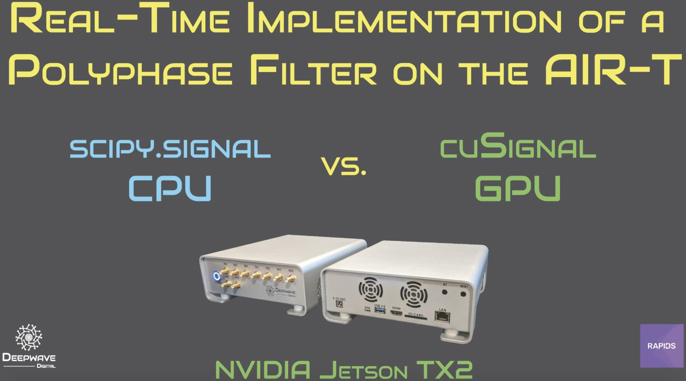
Deepwave has been working with NVIDIA to make online processing of cuSignal a reality. Check out how to perform signal processing in real time in this video.
More advances to come with cuSignal!
As Deepwave continues to help NVIDIA make GPU based signals processing a reality, check back in with us to find out more.
The webinar on March 25, 2020 was a great success and we thank you for attending! The video stream, slides, and source code are now available to the general public.
Available in the new webinar section of our GitHub here.
Original Post
Amid all of the uncertainty in our work schedules, we think now is a great time to host a webinar on signal processing and deep learning with GPUs and the AIR-T. The Webinar will cover the items below but more importantly we will be demonstrating the usage of cuSignal on the AIR-T!
Space is limited so make sure to register in advance. Read below for more information about the webinar and w e hope you will join us!
Deepwave Digital, Inc.
Webinar Agenda
Introduction to Deepwave Digital
We will introduce you to the Deepwave Digital team and provide an overview of what our startup does. We will also discuss the way we see deep learning being applied to systems and signals.
AirStack Programming API for the AIR-T
We will provide a detailed discussion on the application programming interface (API) for the AIR-T, AirStack. The figure below outlines the CPU, GPU, and deep learning interfaces supported.
Demonstrations
Signal Processing Using the GPU on the AIR-T
Here we will discuss programming the embedded NVIDIA Jetson GPU that is part of the AIR-T using CUDA, pyCUDA, and GNU Radio.
cuSignal - NVIDIA's GPU Accelerated Signal Library
cuSignal is an open source GPU accelerated version of Scipy.Signal. The team at NVIDIA started the initiative a few months back and Deepwave has decided to jump on board and contribute. If you are not familiar with cuSignal, it is part of the large RAPIDS project at NVIDIA: the push to GPU accelerate data science libraries.
Finally we will close the webinar by discussing deep learning applications and how to leverage the AIR-T to acquire data and how to deploy trained neural networks on the AIR-T for inference.
If you are looking for a very simple way to acquire the power spectral density of a received signal with the AIR-T, you may like the Soapy Power Project. The resulting spectrum output may be used for monitoring interference, acquiring signals for deep learning, or for examining a test signal. Soapy Power is a part of the larger SoapySDR ecosystem that has built-in support on the AIR-T. In this post, we will walk you through the installation of Soapy Power on the AIR-T and provide a brief demo to help get you started.
Using Soapy Power, it is very easy to acquire a spectrum snapshot and record to a csv file. Sample rate, center frequency, and processing parameters can all be controlled via command-line arguments as you will see in the below example.
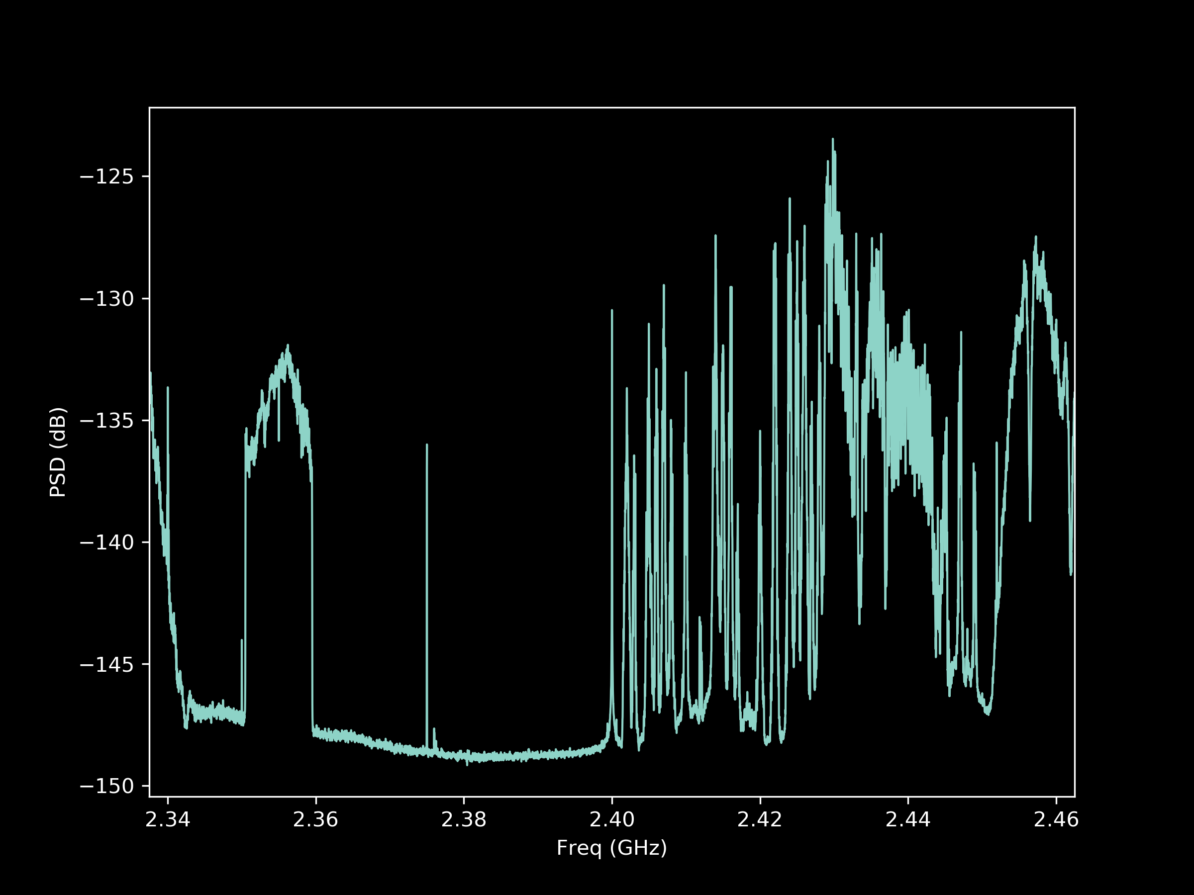
Let's walk through this command. The soapy_power command is the program being called. the -g 0 option sets the gain to 0 dB. The -r 125M option sets the receiver sample rate to 125 MSPS. The -f 2.4G option tunes the radio to 2.4 GHz frequency. We set the FFT size to be 8192 samples using the -b 8192 and average 100 windows using the -n 100 option. Finally, the output file is defined by the -O data.csv option. Following the execution of the above command, a file is recorded with the spectrum data.
To visualize the data, we will use Python's matplotlib package with the following script:
import numpy as npfrom matplotlib import pyplot as pltwith open('data.csv', 'r') as csvfile: data_str = csvfile.read() # Read the datadata = data_str.split(',') # Use comma as the delimitertimestamp = data[0] + data[1] # Timestamp as YYYY-MM-DD hhh:mmm:ssf0 = float(data[2]) # Start Frequencyf1 = float(data[3]) # Stop Frequencydf = float(data[4]) # Frequency Spacingsig = np.array(data[6:], dtype=float) # Signal datafreq = np.arange(f0, f1, df) / 1e9 # Frequency Array# Plot the dataplt.plot(freq, sig)plt.xlim([freq[0], freq[-1]])plt.ylabel('PSD (dB)')plt.xlabel('Freq (GHz)')plt.show()